
TL;DR
Suppose a CNN works well and you can afford more compute. Should you give it more layers, more channels, or larger images? EfficientNet studies how to divide that extra budget. Its compound rule grows all three together, starting from a small searched network called B0.
The important idea is the relationship between the dimensions: more pixels provide extra detail, more channels provide more feature combinations, and more layers let the network transform and combine those features. The following visuals make each change visible before we connect it to the equation and the code. For a published endpoint, B7 reaches 84.3% ImageNet top-1 with 66M parameters in arXiv v5, Table 2.
Why one scaling dimension is insufficient
Think of a CNN as a sequence of feature grids. A grid has a height and width, and each position holds several channels. A channel is a learned feature response; it does not have to correspond to a human-readable category. Layers transform those grids into progressively more useful representations.
There are three ways to make this system bigger:
- Depth: add more transformations along the path from image to prediction.
- Width: give each transformation more input and output channels.
- Resolution: give the network a larger spatial grid to process.
Change one dimension below. The baseline stays visible so you can see exactly where the extra work comes from.
What actually changes when a CNN gets bigger?
Change one dimension in the same small network. Compare the grids, the channel stripes, and the number of layers before looking at the cost.
Baseline
- Multiply–accumulates
- 110,592
- Convolution weights
- 1,728
Double resolution
- Multiply–accumulates
- 442,368
- Convolution weights
- 1,728
Count the cells: doubling both side lengths turns 64 positions into 256. The same filters are evaluated at four times as many places.
Twice the height × twice the width: 4× work, with the same learned weights.
See the paper’s scaling illustration
Notice that doubling a dimension does not have a uniform cost. Doubling depth repeats the work twice. Doubling width grows both the input and output channel dimensions, so a regular convolution costs roughly four times as much. Doubling image side length makes both height and width larger, producing four times as many spatial positions.
The next question is whether that extra work is useful. A larger image can preserve a small object’s details, but the network still has to combine those pixels into features. Its fixed-size filters now cover a smaller fraction of the image. Extra layers can enlarge the receptive field, while extra channels can provide more feature combinations. This is an intuition about how the dimensions interact; the accuracy claim needs an experiment.
What the paper actually tests
Figure 4 varies width under several depth/resolution settings. Each dot is a model; the horizontal axis is reported compute, and the vertical axis is ImageNet accuracy. Read across at a comparable compute budget: the deeper, higher-resolution setting can make better use of width. The useful observation is dependence between the dimensions, rather than an unlimited benefit from making every one larger. Figures 3–4
That motivates a recipe for sharing a budget. First, we need to account for the different prices of depth, width, and resolution.
Compound scaling: an approximation and a recipe
A regular convolution computes one dot product for each output channel at each output position. With kernel side k, that dot product reads k^2 C_{in} values. There are HW C_{out} outputs, giving the multiply–accumulate count:
Now scale a repeated convolutional network. Relative depth d repeats its layers; relative width w grows both channel dimensions; relative resolution r grows both spatial dimensions:
This also explains why a larger image can cost more compute without adding convolution weights: the same filters run at more positions. The toy above counts multiply–accumulates explicitly; the published tables retain the paper’s FLOP convention.
If the budget is about twice the baseline, one possible allocation is depth 2×. Another is width \sqrt{2}×, and another is resolution \sqrt{2}×. All fit the same rough compute constraint, but they produce different networks. EfficientNet chooses smaller increases across all three.
Spend the same estimated compute four ways
Depth, width, and resolution change together in compound scaling. Compare how the same regular-convolution budget is allocated.
Depth only
- Depth
- 1.92×
- Width
- 1.00×
- Resolution
- 1.00×
How the cost is built
1.92×1.00×1.00=1.92×
depth · width² · resolution²
Width only
- Depth
- 1.00×
- Width
- 1.39×
- Resolution
- 1.00×
How the cost is built
1.00×1.92×1.00=1.92×
depth · width² · resolution²
Resolution only
- Depth
- 1.00×
- Width
- 1.00×
- Resolution
- 1.39×
How the cost is built
1.00×1.00×1.92=1.92×
depth · width² · resolution²
Compound
- Depth
- 1.20×
- Width
- 1.10×
- Resolution
- 1.15×
How the cost is built
1.20×1.21×1.32=1.92×
depth · width² · resolution²
The budget is shared, but the networks spend it differently. Compound scaling grows all three dimensions gently instead of assigning the entire increase to one. The paper’s experiments determine which allocation improves accuracy.
What φ and the three coefficients mean
The three coefficients specify how to grow. The compound coefficient φ specifies how far to grow along that chosen recipe:
The paper selects \alpha=1.2,\ \beta=1.1,\ \gamma=1.15 using a small search around the baseline at φ = 1. In that first increment, depth grows 20%, width 10%, and resolution 15%. Because the last two dimensions enter quadratically, the estimated cost becomes:
At φ = 2, the same recipe is applied again: depth is 1.44×, width 1.21×, and resolution 1.3225×. The estimated compute is about 3.69×. Fixing the coefficients turns a three-dimensional search into a path that can be followed toward larger budgets. Equation 3 and Section 4
From a smooth rule to an executable model
A formula can ask for 44.8 channels or 3.6 blocks. A network must choose integers. The released builder rounds channel widths to multiples of eight, with a safeguard against rounding down by more than 10%, and rounds block repeats upward.
For B4, a base width of 32 becomes 32\times1.4=44.8, then rounds to 48. A three-block stage becomes \lceil3\times1.8\rceil=6 blocks. Its released input size is 380. Those choices make B0–B7 discrete presets; their names do not mean φ = 0–7. Original preset builder
The compute rule is approximate for another reason: an EfficientNet contains depthwise convolutions, pooling, channel gates, and fixed input/output dimensions as well as regular convolutions. The powers explain a resource trend; an actual model still needs an operator-level count.
What gets scaled: stem, seven stages, and head
The scaling rule needs a starting architecture. The authors search for B0 using an objective that rewards accuracy while penalizing compute. They then scale that baseline. These are two decisions: which small network to start with, and how to enlarge it. Section 4
B0 begins with a stem convolution, passes through seven MBConv stages, and ends with a classification head. Each stage keeps a common block type and output width. Spatial size shrinks along the network, while the later stages have more channels. Select a model below and follow those two trends on their own axes.
The released architecture, stage by stage
Choose a B-number preset, then follow how spatial size shrinks while channel width grows. The stem and head are separate from the seven MBConv stages.
width 1× · depth 1× · input 224²
- Stem112
- Stage 1112
- Stage 256
- Stage 328
- Stage 414
- Stage 514
- Stage 67
- Stage 77
- Head7
Linear scale · 0 to 112. The selected stage is highlighted.
- Stem32
- Stage 116
- Stage 224
- Stage 340
- Stage 480
- Stage 5112
- Stage 6192
- Stage 7320
- Head1280
Linear scale · 0 to 1280. The selected stage is highlighted.
All stage shapes and repeats
Stem · Conv 3×3
32 × 112 × 112
1 block
Stage 1 · MBConv1
16 × 112 × 112
1 block
Stage 2 · MBConv6
24 × 56 × 56
2 blocks
Stage 3 · MBConv6
40 × 28 × 28
2 blocks
Stage 4 · MBConv6
80 × 14 × 14
3 blocks
Stage 5 · MBConv6
112 × 14 × 14
3 blocks
Stage 6 · MBConv6
192 × 7 × 7
4 blocks
Stage 7 · MBConv6
320 × 7 × 7
1 block
Head · Conv 1×1
1280 × 7 × 7
1 block
Input
16 × 112 × 112Operation
3×3 kernel · first stride 2
Expansion 6× · 2 repeats
Output
24 × 56 × 56A stage’s first block may downsample and change channels. Later blocks keep the stage’s output shape. In B0’s second MBConv stage, the first block takes 16 × 112 × 112 to 24 × 56 × 56. The second takes 24 × 56 × 56 to the same shape, making a residual addition possible. Repetition grows depth without repeatedly halving the grid.
Table 1’s spatial column describes the operator’s input, so the inspector labels both input and output. At the head, B0 has 1280 × 7 × 7 features; B4 has 1792 × 12 × 12. The head has more channels, but it has not produced class probabilities yet. We will return to that final conversion after looking inside MBConv.
Inside MBConv
The name describes an inverted bottleneck. A block starts with a compact feature tensor, creates a wider working space for its nonlinear operations, then projects back to a compact interface. The pointwise convolutions mix channels; the depthwise convolution handles spatial filtering separately in each channel.
Follow a real B0 residual block: 24 × 56 × 56 → 144 × 56 × 56 → 24 × 56 × 56. Step through the visual to see what changes and which connections stay separate.
Follow one MBConv block
Inspect three actual B0 cases. Expansion, stride, and matching channels determine which operations and paths exist.
Input 24 × 56 × 56
Make a wider working space
24 channels
56 × 56 grid
144 channels
56 × 56 grid
A pointwise convolution mixes the input channels into new combinations at every location. Spatial size stays the same.
Plane stacks summarize channel width; square size follows spatial size. Labels give the full tensor shape. No activation values are drawn.
1. Expand
144 × 56 × 56
1×1 · 24 → 144 channels. BN + SiLU.
2. Depthwise
144 × 56 × 56
3×3 · groups 144 · stride 1. BN + SiLU.
3. Reweight
144 × 56 × 56
Global pool 144 channels → squeeze 6 → gates 144. Sigmoid gates multiply the feature grid.
4. Project
24 × 56 × 56
1×1 · 144 → 24 channels. BN, without an activation.
5. Residual decision
24 × 56 × 56
Matching channels and stride 1: add the input. Training applies stochastic depth to the branch.
Expansion and depthwise filtering do different jobs
A 1 × 1 convolution looks at one spatial position and combines its channel values. With expansion six, 24 channels become 144. It adds feature combinations while preserving the 56 × 56 grid. MBConv1 omits this expansion operation.
A depthwise 3 × 3 convolution then gives each expanded channel its own spatial filter. It uses \text{groups}=144, so it does not combine different channels. A dense 3 × 3 convolution from 144 to 144 channels would use 186,624 multiply–accumulates per output position; the depthwise operation uses 1,296. Expansion and projection add their own work, so these counts isolate the spatial operation’s saving.
Expansion and depthwise filtering use batch normalization followed by Swish, implemented as SiLU in the pinned port. The projection has batch normalization with no extra activation. MBConv implementation
A stride-two filter also changes the grid. With dilation one, its output side length is:
For B4’s 95-pixel input to a 5 × 5, stride-two filter with padding two, this gives \lfloor(95+4-5)/2\rfloor+1=48. That is why simply dividing by two and rounding down gives the wrong answer.
Squeeze-and-excitation: one gate per channel
The block pools each 144-channel feature grid to 144 values, one average per channel. A small learned network compresses that descriptor and expands it again to produce 144 sigmoid gates. Each gate multiplies all spatial positions in its own channel. This gives a local feature response a weight informed by the whole feature grid.
The squeeze width is tied to the block’s unexpanded input: \max(1,\lfloor24/4\rfloor)=6. The descriptor therefore follows 144 → 6 → 144. The visual’s planes and connections show this structure; they do not contain measured activations or semantic attention maps.
Projection and the residual path
Projection combines the expanded features into 24 output channels. The result has the original 24 × 56 × 56 shape, so the block can add the unchanged input:
The branch learns a change to the input while the identity path carries the input directly forward. Addition is element-wise, which requires compatible shapes. A block that downsamples or changes the channel count has no identity addition in this implementation. During training, stochastic depth can drop the eligible branch for a sample; evaluation uses the complete branch.
From feature grids to class logits
After all stages, global average pooling turns the B0 head’s 1280 × 7 × 7 grid into a vector of 1280 values. A learned linear classifier maps that vector to 1000 ImageNet logits. Softmax then turns those logits into the displayed distribution over categories. This completes the path from spatial evidence to an image-level prediction.
The implementation below follows that same path, with the original paper reference, tensor math, and Python kept together at every step.
Implementation: paper, math, and Python
The seven rows below follow one executable program. Each keeps the original source connection, the mathematical interpretation, and syntax-highlighted Python visible together. Implementation-specific details cite the torchvision port where the paper leaves them unspecified.
This is an architecture and inference reference. The random-weight smoke mode checks forward/backward mechanics; it does not train a useful classifier. The pretrained mode loads explicit B0/B4 weights strictly and uses their prescribed transforms. It does not reproduce the original TensorFlow training recipe, architecture search, or ImageNet training run.
A tested PyTorch reference follows torchvision 0.27.0. It supports a CPU mechanics check and real pretrained inference. The smoke check uses random weights; it does not reproduce ImageNet training or architecture search.
Download the Python program · Pinned requirements · Reference implementation
python efficientnet.py --smoke --model b0
python efficientnet.py --predict --model b4 --image photo.png
Install with python -m pip install -r requirements-efficientnet.txt. CPU wheels are sufficient. Put the exporter beside this program to reproduce all six saved cases.
1. Turn multipliers into integer channels and repeats
Original paper
Equation 3 gives a smooth growth rule. The released presets turn that rule into whole channels and whole blocks: a feature grid cannot have a fractional channel.
Math and tensor shapes
Width changes how many features each position can hold; depth changes how many times a stage transforms them. Rounding keeps widths aligned to eight. If rounding down would remove more than 10% of the requested width, add another eight. Repeat counts use a ceiling so scaling never requests part of a block.
B4: 32 × 1.4 → 48 channels; 3 × 1.8 → 6 blocks
Python implementation
def round_channels(channels, width_multiplier, divisor=8):
    """Round width while avoiding a reduction greater than ten percent."""
    scaled = channels * width_multiplier
    if scaled <= 0 or divisor <= 0:
        raise ValueError("Channels and divisor must be positive")
    rounded = max(divisor, int(scaled + divisor / 2) // divisor * divisor)
    if rounded < 0.9 * scaled:
        rounded += divisor
    return rounded


def round_repeats(repeats, depth_multiplier):
    """Round each stage's depth upward."""
    if repeats <= 0 or depth_multiplier <= 0:
        raise ValueError("Repeats and depth multiplier must be positive")
    return math.ceil(repeats * depth_multiplier)
2. Assemble the stem, seven stages, and head
Original paper
Table 1 is a stage recipe: choose a block, an output width, and a repeat count. Its resolution column gives the input to that stage. Tan and Le, arXiv v5, Table 1, PDF page 5.
Math and tensor shapes
The first block moves into a new shape. Every later block works within it, using the previous output width as its input width and stride one. This separates spatial downsampling from adding depth. The stem enters the feature network; the head collects the final stage into a wider classification representation.
B0 head: [B, 1280, 7, 7]; B4 head: [B, 1792, 12, 12]
Python implementation
width, depth, _, dropout = PRESETS[model_id]
stem_channels = round_channels(32, width)
layers = [conv_norm(3, stem_channels, kernel=3, stride=2)]
total = sum(round_repeats(s[5], depth) for s in BASE_STAGES)
block_index = 0
for expansion, kernel, stride, cin, cout, repeats in BASE_STAGES:
    cin, cout = round_channels(cin, width), round_channels(cout, width)
    blocks = []
    for repeat in range(round_repeats(repeats, depth)):
        blocks.append(
            MBConv(
                cin if repeat == 0 else cout,
                cout,
                expansion,
                kernel,
                stride if repeat == 0 else 1,
                0.2 * block_index / total,
            )
        )
        block_index += 1
    layers.append(nn.Sequential(*blocks))
head_channels = 4 * round_channels(320, width)
layers.append(conv_norm(round_channels(320, width), head_channels))
self.features = nn.Sequential(*layers)
self.avgpool = nn.AdaptiveAvgPool2d(1)
self.classifier = nn.Sequential(
    nn.Dropout(dropout, inplace=True), nn.Linear(head_channels, 1000)
)
3. Expand channels, then convolve each channel
Original paper
EfficientNet uses mobile inverted bottlenecks. Its spatial operation is depthwise, between two pointwise projections.
Math and tensor shapes
Expansion mixes channels at each position to create a wider working space. Depthwise convolution then filters each expanded channel independently. Setting groups equal to the channel count creates one spatial filter per channel. Both operations use BN and SiLU. With H = 95, p = 2, k = 5, s = 2, the output formula gives 48.
Residual B0 block: [B, 24, 56, 56] → [B, 144, 56, 56]
Python implementation
expanded = round_channels(cin, expansion)
layers = []
if expanded != cin:
    layers.append(conv_norm(cin, expanded, kernel=1))
layers.append(
    conv_norm(
        expanded,
        expanded,
        kernel=kernel,
        stride=stride,
        groups=expanded,
    )
)
layers.append(SqueezeExcitation(expanded, cin))
4. Build a channel gate from global context
Original paper
The paper adds squeeze-and-excitation to its MBConv blocks. The released port supplies the exact bottleneck and activations.
Math and tensor shapes
Pooling summarizes the entire spatial grid without mixing its channels. The small learned network then mixes those summaries to decide one gate per channel. For Cin = 24, the bottleneck is 6 even though the expanded tensor has 144 channels. Broadcasting the gate gives every position in a channel the same multiplier.
144 pooled channels → 6 squeeze channels → 144 gates
Python implementation
class SqueezeExcitation(nn.Module):
    """Gate expanded channels using an input-width squeeze bottleneck."""

    def __init__(self, expanded, input_channels):
        super().__init__()
        squeeze = max(1, input_channels // 4)
        self.avgpool = nn.AdaptiveAvgPool2d(1)
        self.fc1 = nn.Conv2d(expanded, squeeze, 1)
        self.fc2 = nn.Conv2d(squeeze, expanded, 1)
        self.activation = nn.SiLU(inplace=True)
        self.scale_activation = nn.Sigmoid()

    def forward(self, x):
        pooled = self.avgpool(x)
        gates = self.scale_activation(
            self.fc2(self.activation(self.fc1(pooled)))
        )
        return x * gates
5. Project and add the input only when shapes match
Original paper
Inverted residual blocks return to a narrow output. A skip connection is conditional on stride and channel compatibility.
Math and tensor shapes
Projection returns to a compact output width without another activation. When that output matches x, addition gives the branch a direct identity path to build on. Stride two or a changed width breaks that shape match. During training, stochastic depth can drop an eligible branch per sample; evaluation retains it. The excerpt joins the constructor’s final lines to its forward method.
144 → 24 channels; stride 1 permits [B, 24, 56, 56] + x
Python implementation
    layers.append(conv_norm(expanded, cout, activation=False))
    self.block = nn.Sequential(*layers)
    self.use_res_connect = stride == 1 and cin == cout
    self.stochastic_depth = StochasticDepth(drop_probability, "row")

def forward(self, x):
    branch = self.block(x)
    if self.use_res_connect:
        branch = self.stochastic_depth(branch) + x
    return branch
6. Reduce the feature grid to class logits
Original paper
A pointwise head convolution is followed by global pooling and a fully connected classifier.
Math and tensor shapes
Global averaging gives one number per head channel, summarizing that feature across the image. The classifier learns a different weighted combination of those numbers for each category. Its outputs are logits, which cross-entropy consumes directly. Softmax is only needed to display a distribution. Evaluation disables dropout and stochastic depth.
B0: [B, 1280, 7, 7] → [B, 1280] → [B, 1000]
Python implementation
def forward(self, x):
    x = self.features(x)
    x = self.avgpool(x)
    x = torch.flatten(x, 1)
    return self.classifier(x)  # Logits; softmax belongs to the display.
7. Load an explicit checkpoint and preserve its input
Original paper
The pretrained example follows the pinned torchvision port and its explicit IMAGENET1K_V1 weight enums.
Math and tensor shapes
The checkpoint and transform are a pair: training determined which normalized inputs these weights expect. Select an explicit enum, load its tensors strictly, and preserve the crop before subtracting the RGB means and dividing by the standard deviations. Keeping that crop lets the reader inspect exactly what reached the classifier.
B0 crop: [1, 3, 224, 224]; B4 crop: [1, 3, 380, 380]
Python implementation
def load_pretrained(model_id):
    """Strictly load the released port; weights are cached outside this repo."""
    weights = get_weights(model_id)
    model = build_efficientnet(model_id)
    model.load_state_dict(
        weights.get_state_dict(progress=False, check_hash=True), strict=True
    )
    return model.cpu().float().eval(), weights


def prepare_image(image, weights_enum):
    """Keep the exact PIL crop and normalized tensor together."""
    transform = weights_enum.transforms()
    image = image.convert("RGB")
    resized = F.resize(
        image,
        transform.resize_size,
        interpolation=transform.interpolation,
        antialias=transform.antialias,
    )
    crop = F.center_crop(resized, transform.crop_size)
    tensor = F.convert_image_dtype(F.pil_to_tensor(crop), torch.float32)
    batch = F.normalize(tensor, transform.mean, transform.std).unsqueeze(0)
    size = transform.crop_size[0]
    left = int(round((resized.width - size) / 2))
    top = int(round((resized.height - size) / 2))
    record = {
        "resizeSize": transform.resize_size[0],
        "cropSize": size,
        "interpolation": "bicubic",
        "antialias": transform.antialias,
        "mean": transform.mean,
        "std": transform.std,
        "resizedShape": [resized.height, resized.width],
        "cropBox": [left, top, left + size, top + size],
    }
    return crop, batch, record
The head row separates a model’s 1000 logits from the softmax used to display predictions. We can now use that exact program with released weights and inspect the inputs as well as the outputs.
Real pretrained example: B0 versus B4
Both checkpoints see the same source photograph, but their prescribed preprocessing retains different crop fractions. Showing both actual crops keeps that difference visible. The three photographs demonstrate inference; they are not an evaluation dataset or evidence that B4 always predicts better.
One photograph, two pretrained models
These are saved CPU inference results from strictly loaded ImageNet-1K V1 checkpoints. Select a photograph and follow the same stage through both networks.
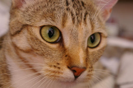
Showing B0 and B4 for Chelsea the cat.
B0 resizes the shorter edge to 256 and center-crops 224; B4 resizes to 384 and center-crops 380. They retain different crop fractions. Both exact RGB crops are shown below, before normalization. This is a comparison of two pretrained packages, not a controlled resolution ablation.
EfficientNet-B0
5,288,548 parameters · 224 × 224 input
EfficientNet_B0_Weights.IMAGENET1K_V1
Top five · softmax probability
- Egyptian cat57.47%
- tiger cat24.39%
- tabby12.29%
- lynx0.20%
- swab0.07%
Stage 3 · measured shape
Input 1 × 24 × 56 × 56
Output 1 × 40 × 28 × 28
Kernel 5 × 5 · first stride 2 · 2 blocks
Batch × channels × height × width; classifier tensors use batch × features.
EfficientNet-B4
19,341,616 parameters · 380 × 380 input
EfficientNet_B4_Weights.IMAGENET1K_V1
Top five · softmax probability
- Egyptian cat46.28%
- tabby9.09%
- tiger cat7.58%
- lynx2.89%
- plastic bag0.17%
Stage 3 · measured shape
Input 1 × 32 × 95 × 95
Output 1 × 56 × 48 × 48
Kernel 5 × 5 · first stride 2 · 4 blocks
Batch × channels × height × width; classifier tensors use batch × features.
Weights, preprocessing, and reproduction
Exported 2026-10-10T05:10:10.674707+00:00. CPU float32, 2 threads; PyTorch 2.12.0+cu130, torchvision 0.27.0+cu130, Pillow 12.2.0. Saved crops reconstruct the normalized tensors exactly. The authored model agrees with torchvision on all six runs, with maximum absolute logit error 0.
EfficientNet_B0_Weights.IMAGENET1K_V1
Checkpoint (21,444,401 bytes)SHA256: 7f5810bc96def8f7552d5b7e68d53c4786f81167d28291b21c0d90e1fca14934
Bicubic PIL resize, antialiasing enabled; mean [0.485, 0.456, 0.406], std [0.229, 0.224, 0.225].
EfficientNet_B4_Weights.IMAGENET1K_V1
Checkpoint (78,107,389 bytes)SHA256: 23ab8bcd5bdbef61a7a43b91adcad81f622fd7f36fb4935a569828d77888c44e
Bicubic PIL resize, antialiasing enabled; mean [0.485, 0.456, 0.406], std [0.229, 0.224, 0.225].
Current photograph: Stefan van der Walt · CC0. Original PNG. All three photographs and their credits are recorded in the full export.

Model source SHA256: 54b4ec3322b21ab6dd633da906bd8d93d619b942b11bcd106c650df011720308
Exporter SHA256: 9a39a4bb64526bfb1de7021f1d11f1a92a769715f7363b972d54c3d050ee77c5
Full measured resultsReproduce the exportPinned requirements
The astronaut is a useful reminder of the label space: B0’s top result is “crash helmet,” while B4’s is “space shuttle.” Neither supplies an “astronaut” category. A high softmax probability is not a guarantee that a label describes the image well, and a larger model need not provide the more helpful answer on every photograph.
Those observations are measured outputs of particular checkpoints. The paper’s dataset-level results answer a different question: how does the family trade accuracy against model size and reported compute?
Published results and their protocols
The family table below uses arXiv:1905.11946v5, Table 2 consistently. Its ImageNet validation comparisons exclude ensemble, multi-crop, and Instagram-pretrained models. The ICML proceedings version contains different accuracy values, so numbers from the two versions should not be mixed.
| Model | Top-1 (%) | Parameters (M) | FLOPs (B) |
|---|---|---|---|
| B0 | 77.1 | 5.3 | 0.39 |
| B1 | 79.1 | 7.8 | 0.7 |
| B2 | 80.1 | 9.2 | 1 |
| B3 | 81.6 | 12 | 1.8 |
| B4 | 82.9 | 19 | 4.2 |
| B5 | 83.6 | 30 | 9.9 |
| B6 | 84.0 | 43 | 19 |
| B7 | 84.3 | 66 | 37 |
B7’s 84.3% matches the GPipe result listed in Table 2 while using 66M rather than 557M parameters, about 8.4 times fewer. That table does not provide GPipe’s FLOPs. The paper’s “6.1× faster” comparison comes from a separate latency measurement, not a FLOP ratio. Tables 2 and 4
Published CPU latency
Table 4 measures batch size one on a single core of an Intel Xeon E5-2690, averaged over 20 runs. It reports these times:
| Model | Seconds per image |
|---|---|
| ResNet-152 | 0.554 |
| EfficientNet-B1 | 0.098 |
| GPipe | 19 |
| EfficientNet-B7 | 3.1 |
These yield the reported 5.7× B1-versus-ResNet-152 and 6.1× B7-versus-GPipe CPU speedups. They are not GPU results or timings from our exporter. Table 4 also lists B1/B7 accuracies of 78.8%/84.4%, which differ from Table 2’s 79.1%/84.3% in the same PDF. We retain Table 2 for the accuracy table and identify Table 4 solely as the latency source. Table 4 and Section 5.2
The distinction matters in practice: fewer reported FLOPs can help, but operator kernels, memory traffic, batch size, and hardware determine elapsed time. An architectural estimate and a timed experiment are different evidence.
Critical analysis
The useful contribution is a compact hypothesis about balanced growth, tested across a searched baseline and other CNNs. It gives a starting point for allocating additional compute without independently guessing three dimensions.
Its limits follow from the same construction. The regular-convolution approximation does not count every operator precisely. Channel rounding and integer repeats make released models discrete. Coefficients selected at one budget are not guaranteed to remain optimal at every larger budget. And EfficientNet’s strong B0 architecture is part of the result: the scaling rule alone does not explain every gain over earlier networks.
For deployment, parameter count, FLOPs, memory use, and latency should be checked separately on the intended device. The CPU protocol above cannot establish a contemporary GPU or edge-device speedup. For these pretrained examples, preprocessing and checkpoint training also contribute to the outcome, so the B0/B4 comparison does not isolate architectural scale.
These limits suggest the next extension: optimize the training process and operator choices alongside model size.
From EfficientNet to EfficientNetV2
EfficientNetV2 makes training speed an explicit search objective and adds Fused-MBConv to the search space. It also progressively increases image size while adapting regularization. These are later changes to the architecture and training method, not hidden parts of the 2019 MBConv implementation above.
EfficientNet’s broader lesson remains useful when thinking about scaling laws: increasing a resource budget requires deciding how to divide it among interacting dimensions. The appropriate dimensions and empirical rule depend on the model and task.
Takeaways
The scaling equation explains the allocation, the stage map explains the discrete network, and the annotated code exposes the operations and branch conditions. The real B0/B4 example then shows how explicit weights and preprocessing produce observable outputs. Published accuracy and CPU timing belong to their own benchmark protocols.
When using this family, start with a released preset, preserve its expected transform, and measure the resource that matters for your workload. The downloadable program and full exported vectors make the small inference comparison reproducible.
Related Reading
- Deep Residual Learning: skip connections and the value of depth.
- Vision Transformer: patch-based transformers and a different scaling approach.
- Swin Transformer: hierarchical vision transformers at several scales.
- YOLO: detection workloads where backbone efficiency affects latency.
- DINO: self-supervised learning with vision backbones.