
TL;DR
ViT demonstrates that a standard Transformer encoder, applied directly to sequences of image patches, can match or exceed the best convolutional networks on image classification — provided it is pre-trained on sufficient data. The architecture is deliberately minimal: split an image into 16x16 patches, linearly embed each patch, prepend a learnable classification token, add positional embeddings, and feed the sequence through a vanilla Transformer. When pre-trained on JFT-300M (300 million images), ViT-Huge/14 reaches 88.55% top-1 accuracy on ImageNet, surpassing the best CNNs while using fewer compute resources to train.
The Core Idea: Image Patches as Tokens
The central insight is a reframing: treat an image not as a pixel grid but as a sequence of patch tokens, then apply the same Transformer architecture that works for language. This is a deliberate bet on scale over inductive bias. CNNs bake in locality (convolution kernels) and translation equivariance (weight sharing) — priors that help with limited data. ViT discards both, relying instead on the Transformer's capacity to learn these relationships from data when given enough of it.
An input image \mathbf{x} \in \mathbb{R}^{H \times W \times C} is reshaped into a sequence of N flattened patches \mathbf{x}_p \in \mathbb{R}^{N \times (P^2 \cdot C)}, where P is the patch size and N = HW / P^2. For a 224x224 image with 16x16 patches, this yields N = 196 tokens — a sequence length easily handled by a Transformer.
Patch Embedding
Each flattened patch is projected into the model's hidden dimension D through a learnable linear projection:
In practice this is implemented as a single convolution with kernel size and stride both equal to P, which is mathematically equivalent to flattening plus linear projection but more efficient on GPU hardware.
A learnable [CLS] token \mathbf{z}_0^0 is prepended to the patch sequence, following the BERT convention. Its output representation at the final layer serves as the aggregate image representation for classification. Learnable 1D positional embeddings \mathbf{E}_{pos} \in \mathbb{R}^{(N+1) \times D} are added to the full sequence to encode spatial information:
The paper found that learned 1D positional embeddings perform comparably to more sophisticated 2D-aware alternatives, suggesting the model learns to infer spatial structure from the data.
Transformer Encoder
The patch embeddings are processed by a standard Transformer encoder — the same architecture from Vaswani et al. (2017), with no vision-specific modifications. Each of the L layers applies multihead self-attention (MSA) followed by an MLP block, both with layer normalization applied before each block (pre-norm) and residual connections:
The MLP contains two linear layers with a GELU activation. The output of the [CLS] token at the final layer is passed through a classification head (a single linear layer during fine-tuning) to produce the class prediction:
Self-attention allows every patch to attend to every other patch at every layer, giving the model a global receptive field from the first layer. This contrasts with CNNs, where the effective receptive field grows linearly with depth.
Pre-training at Scale
ViT's central experimental finding is that dataset scale determines whether the architecture succeeds or fails. When trained from scratch on ImageNet-1k (1.3M images), ViT-Base performs several points below a comparably sized ResNet. The Transformer lacks the inductive biases that let CNNs generalize from limited data. But this deficit inverts with scale:
- ImageNet-21k (14M images): ViT becomes competitive with CNNs.
- JFT-300M (300M images): ViT surpasses the best CNNs at lower total training compute.
The paper pre-trains on these large datasets using standard supervised classification, then fine-tunes on downstream tasks. Pre-training uses Adam with a learning rate warmup; Table 3 specifies linear decay for JFT and ImageNet-21k, and cosine decay for ImageNet-1k. The large-scale pre-training essentially substitutes for the missing inductive biases — what locality and translation equivariance give CNNs for free, ViT learns from data.
Fine-tuning Strategy
For fine-tuning on downstream tasks, the pre-trained classification head is replaced with a zero-initialized linear layer sized for the target number of classes. A key practical detail: fine-tuning at higher resolution than pre-training improves performance. When the input resolution increases, the number of patches grows (e.g., from 196 at 224px to 576 at 384px), so the pre-trained positional embeddings are 2D-interpolated to the new grid size. This works well in practice despite the positional embeddings being learned as 1D vectors.
Fine-tuning uses SGD with momentum, lower learning rates than pre-training, and typically runs for only a few thousand steps — far less compute than pre-training.
Implementation
The architecture and fine-tuning rules above now fit into one forward pass. Read each original paper reference beside its equations, tensor shapes, and the corresponding Python. For ViT-B/16, a batch of RGB images becomes 196 patch tokens plus CLS, passes through twelve encoder blocks, and ends in 1,000 class logits.
Follow the original equations into one executable PyTorch program. The tiny CPU check uses random weights; the photo example loads a real ViT-B/16 checkpoint into the same authored architecture.
Python program · Pinned requirements · Photo result exporter
python -m pip install -r requirements-vit.txt
python vit.py --smoke
python vit.py --predict --image photo.png --output-dir prediction
CPU wheels are sufficient. Prediction downloads about 330 MB once and caches the weights. The displayed excerpts and syntax colors are generated from the tested downloadable file.
1. Project each patch into a token
Original paper
The paper projects flattened image patches into a common hidden width. The convolution below performs the same linear map, with the bias used by the released implementations.
Math and tensor shapes
Kernel size and stride both equal P, so patches do not overlap. Flattening the two grid axes produces row-major tokens. Within a patch, PyTorch uses channel, row, column order; a flattened linear projection must use that same order. Rejecting an unexpected image size prevents partial patches from being silently discarded.
[B, 3, 224, 224] → [B, 768, 14, 14] → [B, 196, 768]
Python implementation
def patch_tokens(self, images):
    if images.ndim != 4 or images.shape[1] != 3:
        raise ValueError("Expected RGB images with shape [B, 3, H, W]")
    if tuple(images.shape[-2:]) != (self.image_size, self.image_size):
        raise ValueError(
            "Use the configured image size; resize positions when fine-tuning"
        )
    # Conv2d uses channel/row/column order within each flattened patch.
    grid = self.conv_proj(images)
    return grid.flatten(2).transpose(1, 2)  # [B, N, D], row-major patches
2. Prepend CLS and add learned positions
Original paper
A learned classification token occupies slot zero. Learned position vectors are added to the full sequence, including that slot.
Math and tensor shapes
expand shares the same learnable CLS vector across the batch without creating independent parameters. Concatenation adds one token, then broadcasting adds a different learned vector at every sequence position. The encoder applies dropout to this combined input during training.
[B, 196, 768] → [B, 197, 768]; E_pos: [1, 197, 768]
Python implementation
def embed_tokens(self, patches):
    cls = self.class_token.expand(patches.shape[0], -1, -1)
    tokens = torch.cat([cls, patches], dim=1)
    return tokens + self.encoder.pos_embedding  # [B, N+1, D]
3. Make the attention axes explicit
Original paper
Each head computes a distribution over the input tokens. The heads run in parallel, then their concatenated outputs are projected back to the model width.
Math and tensor shapes
The packed projection is split into three tensors and twelve heads. Scaling by the square root of the head width keeps dot products in a useful range. Softmax runs over the key axis, so every query has its own distribution. CLS participates in the same attention as the image patches. This readable version materializes the attention matrix; optimized kernels can avoid that allocation.
Q, K, V: [B, 12, 197, 64]; A: [B, 12, 197, 197]
Python implementation
class SelfAttention(nn.Module):
    """Expose the Q/K/V and head axes; keep released checkpoint key names."""

    def __init__(self, hidden_dim, num_heads, dropout=0.0):
        super().__init__()
        if hidden_dim % num_heads:
            raise ValueError("Hidden width must be divisible by head count")
        self.num_heads = num_heads
        self.in_proj_weight = nn.Parameter(
            torch.empty(3 * hidden_dim, hidden_dim)
        )
        self.in_proj_bias = nn.Parameter(torch.zeros(3 * hidden_dim))
        self.out_proj = nn.Linear(hidden_dim, hidden_dim)
        self.dropout = nn.Dropout(dropout)
        nn.init.xavier_uniform_(self.in_proj_weight)
        nn.init.zeros_(self.out_proj.bias)

    def forward(self, x):
        batch, tokens, width = x.shape
        head_dim = width // self.num_heads
        qkv = F.linear(x, self.in_proj_weight, self.in_proj_bias)
        qkv = qkv.reshape(batch, tokens, 3, self.num_heads, head_dim)
        q, k, v = qkv.permute(2, 0, 3, 1, 4).unbind(0)
        scores = (q @ k.transpose(-2, -1)) / math.sqrt(head_dim)
        weights = self.dropout(scores.softmax(dim=-1))
        attended = (weights @ v).transpose(1, 2).reshape(batch, tokens, width)
        return self.out_proj(attended)
4. Normalize each branch before adding its residual
Original paper
Layer normalization comes before attention and before the MLP. Both branch outputs are added to their respective inputs.
Math and tensor shapes
The skip path keeps the unnormalized input. The MLP acts independently on each token, mixing its channels with Linear, GELU, then Linear. Attention mixes tokens; the MLP mixes channels. Twelve blocks repeat this pattern for ViT-B/16. LayerNorm uses the pinned port’s epsilon of 1e-6.
All block inputs/outputs: [B, 197, 768]; MLP width: 768 → 3072 → 768
Python implementation
class EncoderBlock(nn.Module):
    """Pre-normalize each branch; add its result to the unnormalized residual."""

    def __init__(self, width, heads, mlp_dim, dropout, attention_dropout):
        super().__init__()
        self.ln_1 = nn.LayerNorm(width, eps=1e-6)
        self.self_attention = SelfAttention(width, heads, attention_dropout)
        self.dropout = nn.Dropout(dropout)
        self.ln_2 = nn.LayerNorm(width, eps=1e-6)
        self.mlp = nn.Sequential(
            nn.Linear(width, mlp_dim),
            nn.GELU(),
            nn.Dropout(dropout),
            nn.Linear(mlp_dim, width),
            nn.Dropout(dropout),
        )

    def forward(self, x):
        x = x + self.dropout(self.self_attention(self.ln_1(x)))
        return x + self.mlp(self.ln_2(x))
5. Read the final CLS feature and predict classes
Original paper
Equation 4 defines the normalized CLS representation. The classification head consumes that representation; its form differs between the paper’s pre-training and fine-tuning.
Math and tensor shapes
The encoder applies its final LayerNorm token by token, and slot zero becomes the image feature. The default head is linear, as in fine-tuning and this released checkpoint. Passing representation_size enables the paper-style one-hidden-layer pre-training head with tanh. Return raw logits; a softmax is only needed to display probabilities.
[B, 197, 768] → [B, 768] → [B, 1000]
Python implementation
def forward(self, images):
    patches = self.patch_tokens(images)
    tokens = self.embed_tokens(patches)
    encoded = self.encoder(tokens)  # L blocks, then final LayerNorm
    image_feature = encoded[:, 0]  # CLS, not the mean of patch tokens
    return self.heads(image_feature)  # Raw class logits
6. Take a supervised training step
Original paper
ViT uses labeled classification for pre-training and downstream fine-tuning. The paper fine-tunes with SGD and momentum; a new downstream head starts at zero.
Math and tensor shapes
Cross-entropy accepts logits directly and handles the log-softmax internally. Clear old gradients, backpropagate, clip the global norm, then update. With a zero head, the first update changes the classifier; gradients reach the backbone on the next update. The smoke command runs two steps on random pixels to expose this mechanics. It does not implement large-scale data loading, augmentation, or learning-rate scheduling.
Images: [B, 3, H, W]; labels: [B]; loss: scalar
Python implementation
def training_step(model, images, labels, optimizer):
    """One supervised update; scheduling and real datasets belong to the caller."""
    model.train()
    optimizer.zero_grad(set_to_none=True)
    logits = model(images)
    loss = F.cross_entropy(logits, labels)  # Do not apply softmax first.
    loss.backward()
    nn.utils.clip_grad_norm_(model.parameters(), max_norm=1.0)
    optimizer.step()
    return loss.detach().item()
7. Resize the position grid for fine-tuning
Original paper
Equation 1 contains the learned position table. Section 3.2 resizes its patch positions according to their original two-dimensional locations when the image resolution changes.
Math and tensor shapes
Separate CLS before restoring the spatial grid. Interpolate that grid, flatten it back to the same row-major order, and put the untouched CLS position first. Bilinear interpolation with aligned corners follows the authors’ order-1 grid resize. A resolution change also requires constructing the model at the new image size, loading the resized position table, and fine-tuning it; the pretrained prediction below retains its prescribed 224px crop.
224 → 384 px, P=16: [1, 197, 768] → [1, 577, 768]
Python implementation
def resize_positions(positions, old_grid, new_grid):
    """Bilinearly resize patch positions, leaving the CLS position untouched."""
    if any(
        len(grid) != 2 or any(not isinstance(n, int) or n <= 0 for n in grid)
        for grid in (old_grid, new_grid)
    ):
        raise ValueError(
            "Position grids must contain two positive integer sizes"
        )
    if positions.ndim != 3 or positions.shape[0] != 1:
        raise ValueError("Expected positions with shape [1, N+1, D]")
    if positions.shape[1] != old_grid[0] * old_grid[1] + 1:
        raise ValueError(
            "Old grid does not match the number of patch positions"
        )
    cls_position, patch_positions = positions[:, :1], positions[:, 1:]
    grid = patch_positions.reshape(1, *old_grid, positions.shape[-1])
    grid = grid.permute(0, 3, 1, 2)
    grid = F.interpolate(
        grid, size=new_grid, mode="bilinear", align_corners=True
    )
    resized = grid.flatten(2).transpose(1, 2)
    return torch.cat([cls_position, resized], dim=1)
8. Load a real checkpoint and keep its exact input
Original paper
The real example uses torchvision’s explicitly named ViT-B/16 ImageNet-1k weights. The original authors’ public JAX checkpoints are a separate release.
Math and tensor shapes
Load all checkpoint tensors strictly, including an explicit migration of the released V1 MLP names. Use the weight enum’s bilinear resize, center crop, and RGB normalization. Keep the actual crop beside the prediction so readers can inspect what reached the model. Evaluation disables dropout, and inference_mode avoids recording gradients.
RGB → shorter edge 256 → center crop 224 → [1, 3, 224, 224]
Python implementation
def load_pretrained():
    """Load an explicit ImageNet-1k checkpoint into this authored architecture."""
    weights = ViT_B_16_Weights.IMAGENET1K_V1
    model = VisionTransformer()
    state = weights.get_state_dict(progress=True, check_hash=True)
    model.load_state_dict(checkpoint_keys(state), strict=True)
    return model.cpu().float().eval(), weights


def prepare_image(image, weights):
    """Return exactly what the checkpoint sees, before and after normalization."""
    transform = weights.transforms()
    resized = TF.resize(
        image.convert("RGB"),
        transform.resize_size,
        interpolation=transform.interpolation,
        antialias=transform.antialias,
    )
    crop = TF.center_crop(resized, transform.crop_size)
    pixels = TF.convert_image_dtype(TF.pil_to_tensor(crop), torch.float32)
    batch = TF.normalize(pixels, transform.mean, transform.std).unsqueeze(0)
    return crop, batch


@torch.inference_mode()
def predict(model, weights, image):
    crop, batch = prepare_image(image, weights)
    logits = model(batch)
    scores, indices = logits.softmax(dim=-1)[0].topk(5)
    top5 = [
        {
            "index": int(i),
            "label": weights.meta["categories"][int(i)],
            "score": float(s),
        }
        for s, i in zip(scores, indices)
    ]
    return crop, batch, logits, top5
Check the mechanics on CPU
The --smoke command uses a smaller configuration: 32px images, 4px patches, a hidden width of 64, and two encoder blocks. It reports [2, 64, 64] patch embeddings, [2, 65, 64] tokens, and [2, 10] logits, then takes two supervised updates and resizes the position grid from 8×8 to 12×12. This exercises the same operations as ViT-B/16 without downloading weights or claiming useful accuracy from random pixels.
Classify real photos with pretrained ViT-B/16
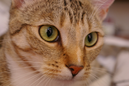
The next examples use the full architecture and released weights. Compare each photograph with the exact crop used before normalization, then read the model’s top five predictions.
These are saved CPU predictions from ViT_B_16_Weights.IMAGENET1K_V1, trained on ImageNet-1k with a modified DeiT recipe. They illustrate usable image classification; they do not reproduce the paper’s JFT pre-training results. Softmax scores express the model’s distribution over its 1,000 classes, rather than calibrated certainty.
Chelsea the cat
Top five predictions
- Egyptian cat66.07%
- tiger cat9.84%
- tabby8.79%
- lynx0.22%
- feather boa0.06%
Photo: Stefan van der Walt · CC0 source · Download the original
Cup of coffee
Top five predictions
- espresso90.31%
- cup1.09%
- coffee mug0.16%
- tray0.12%
- espresso maker0.07%
Photo: Rachel Michetti · CC0 source · Download the original

Keep vit_export.py beside vit.py and run python vit_export.py --output-dir vit-demo to reproduce both cases. It checks the source photos, exact preprocessing, and every output logit against torchvision’s reference model. Inspect the measured outputs and checkpoint provenance.
Pinned PyTorch reference · Original authors’ JAX code and checkpoints
The operations stay the same across ViT sizes. What changes is the depth, hidden width, number of heads, and patch size, which determine the memory and computation in each stage.
ViT Variants
The paper defines three model configurations following the naming convention Model/Patch-size:
| Variant | Layers | Hidden dim D | MLP dim | Heads | Params |
|---|---|---|---|---|---|
| ViT-Base/16 | 12 | 768 | 3072 | 12 | 86M |
| ViT-Large/16 | 24 | 1024 | 4096 | 16 | 307M |
| ViT-Huge/14 | 32 | 1280 | 5120 | 16 | 632M |
The "/16" or "/14" suffix denotes patch size. Smaller patches mean more tokens (longer sequences) and proportionally more compute due to the quadratic cost of self-attention, but they also capture finer spatial detail. ViT-H/14 uses 14x14 patches, yielding 256 tokens for a 224px image compared to 196 tokens for 16x16 patches.
Key Results
When pre-trained on JFT-300M, ViT achieves state-of-the-art results across multiple benchmarks:
- ImageNet: 88.55% top-1 (ViT-H/14), surpassing the previous best of 87.4% (EfficientNet-L2 with Noisy Student) while requiring 2.5x less compute to pre-train.
- CIFAR-100: 94.55% top-1.
- VTAB (19-task suite): Highest average across all three task groups (Natural, Specialized, Structured).
The compute efficiency result is notable: ViT reaches a given accuracy level with fewer training FLOPs than CNN baselines like BiT (Big Transfer). The scaling curves show that ViT performance has not saturated at JFT-300M scale, suggesting further gains with larger datasets.
The Data Efficiency Problem
ViT's reliance on large-scale pre-training is its most significant practical limitation. Without JFT-300M (a proprietary Google dataset), reproducing the top results is infeasible. On ImageNet-1k alone, ViT-Base underperforms a ResNet-50 trained with modern regularization. The reason is structural: a Transformer must learn from data what convolutions encode by design — that nearby pixels are more relevant than distant ones, and that patterns are translation-invariant.
This gap motivated substantial follow-up work. DeiT (Touvron et al., 2021) showed that with aggressive data augmentation (RandAugment, Mixup, CutMix), regularization (stochastic depth, repeated augmentation), and a distillation token trained against a CNN teacher, ViT-Base can reach 81.8% on ImageNet-1k using only that dataset. This demonstrated that ViT's data hunger is not fundamental but can be addressed through training recipes that partially compensate for the missing inductive biases.
Critical Analysis
Strengths:
- Architectural simplicity. ViT applies a standard NLP Transformer to vision with essentially zero domain-specific modifications. This simplicity enables direct transfer of advances in Transformer scaling, training techniques, and hardware optimization.
- Favorable scaling behavior. Performance improves log-linearly with compute and data, and the scaling curves show no signs of saturation. This is a strong argument for the architecture's long-term viability.
- Transfer learning. A single pre-trained ViT transfers well across diverse downstream tasks with minimal fine-tuning, making it a practical foundation model.
Limitations:
- No locality inductive bias. The global self-attention mechanism treats all patches equally regardless of spatial proximity. This hurts data efficiency and makes the model rely on large datasets to learn spatial relationships that CNNs encode structurally.
- Quadratic attention cost. Self-attention scales as O(N^2) with sequence length, making high-resolution inputs expensive. A 224px image with 16x16 patches produces 196 patch tokens, but moving to 14x14 patches at 378px yields 729 patch tokens — about a 14x increase in attention computation.
- Positional embedding limitations. The learned 1D positional embeddings require interpolation for resolution changes and do not generalize to drastically different aspect ratios or image sizes without fine-tuning.
- Pre-training data requirements. The flagship results depend on JFT-300M, a dataset that is not publicly available, limiting reproducibility.
Impact and Legacy
ViT's impact on computer vision has been substantial, not because it was the first to apply attention to images, but because it demonstrated that a pure Transformer — with no convolutional layers — could work at scale. This shifted the field's default architecture away from CNNs.
Direct architectural descendants include the Swin Transformer (Liu et al., 2021), which reintroduces locality through shifted windows and hierarchical feature maps, achieving strong performance on dense prediction tasks where ViT struggles. DeiT showed that careful training recipes could close the data gap on ImageNet-1k.
Self-supervised learning adopted ViT as the standard backbone. DINO (Caron et al., 2021) demonstrated that ViT trained with self-distillation learns features that explicitly encode semantic segmentation without supervision. MAE (He et al., 2022) showed that masking 75% of patches and reconstructing them produces strong representations, achieving 87.8% on ImageNet with ViT-Huge. BEiT (Bao et al., 2022) adapted BERT-style pre-training to vision patches.
Multimodal models built directly on ViT. CLIP (Radford et al., 2021) trains a ViT image encoder alongside a text encoder via contrastive learning, producing zero-shot classifiers that generalize across distributions. The ViT encoder is now a standard component in models like LLaVA and BLIP-2, though not a universal one: Flamingo uses a contrastively pretrained NFNet-F6, a convolutional network.
Related Reading
- Attention Is All You Need — the original Transformer architecture that ViT applies directly to vision
- Deep Residual Learning — ResNet, the CNN baseline that ViT aims to surpass at scale
- DINO — self-supervised training of ViT that reveals emergent segmentation in attention maps
- MAE — masked autoencoding pre-training for ViT, reducing dependence on labeled data
- BEiT — BERT-style pre-training adapted for vision transformers
- CLIP — contrastive language-image pre-training using ViT as the visual encoder
- Swin Transformer — hierarchical vision transformer with shifted windows, addressing ViT's limitations on dense tasks